Interpretability
Discussion on Interpretability
AIBMod has spent considerable time and effort developing an interpretable framework for the model.
This was a critical success factor for the development project.
Early on, AIBMod realised that there were two parts to the interpretability problem:
- Feature Sensitivity – How sensitive is a prediction to changes in the feature values, and
- Feature Importance – Given the feature values, which of the feature values are key to the prediction.
These are two very different problems but conceptually often become conflated.
In order to establish the answer to the first question it’s a reasonably simple matter of changing, one at a time, each of the feature values to a new one and rerunning the model and calculating the prediction change. For categorical values this is straightforward. This is slightly more involved for numerical values – AIBMod has developed a method for coming up with meaningful numerical buckets to cycle through.
The second question is much more complicated and requires a model to be able to give meaningful predictions when features are removed. AIBMod has developed both a model and training framework to enable this to occur.
The AIBMod Feature Importance analysis is similar in nature to Shapley analysis but is considerably more efficient to produce and gives a bespoke analysis for an individual prediction and how the features drive it. Furthermore, the Feature Importance ‘engine’ is created as part of the model training process – there is not one model for predictions and another to produce the Feature Importance analysis – they are one and the same.
The examples below relate to two predictions from the Adult Income (AD) dataset. This dataset is an extract from the 1994 US Census and the machine learning problem is to build a model that can predict if an individual earns over $50,000 (Class 1).
In addition, the Class 1 probabilities for the examples below were derived using the model whose results can be seen here.
| Categorical Features | workclass | education | marital_status | occupation | relationship | race | gender | native_country |
| Example 1 | Private | 10th | Never-married | Other-service | Not-in-family | White | Male | United-States |
| Example 2 | Self-emp-inc | Assoc-acdm | Married-civ-spouse | Craft-repair | Husband | White | Male | United-States |
| Numerical Features | age | fnlwgt | educational_num | capital_gain | capital_loss | hours_per_week |
| Example 1 Cont. | 34 | 198693 | 6 | nan | nan | 34 |
| Example 2 Cont. | 41 | 445382 | 12 | 15024 | nan | 60 |
| AIBMod Class 1 Probability | Actual Class | |
| Example 1 Cont. | 0.3193% | 0 |
| Example 2 Cont. | 98.6418% | 1 |
So, the eternal machine learning question is why does the model say example 1 is almost certainly not earning over $50,000? Which feature values are driving the prediction and which are irrelevant?
And the same questions for example 2 – why does the model say this individual is almost certainly earning over $50,000?
The feature importance framework that AIBMod has developed answers these questions.
Feature Importance Analysis Example 1 – Adult Income
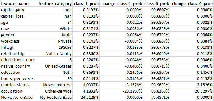
Discussion Of Above
The analysis above was produced with the very model that gave the overall test results for the Adult Income dataset (AD) here. It seeks to answer the question, which features are unimportant, or less relevant, to the overall prediction and which are important?
The top row shows the overall prediction – namely the probability of this individual earning over $50,000 per annum (Class 1) – of 0.3193%.
So very unlikely.
In fact, the individual is in Class 0 so the model has made a good prediction.
The last row shows the base prediction, namely, if one knew nothing about the individual it should be the class 1 probability from the training dataset.
The model has learned a probability of 24.5129% vs the actual training dataset Class 1 probability of 24.081%.
Looking down the table shows the impact to the class 1 probability of removing the feature indicated in the first two columns.
The table has been constructed by first removing the features which give the smallest impact on the Class 1 probability. Hence, this approach leaves the most important features towards the end of the list.
The penultimate row shows that if all one knows about the individual is that their occupation is ‘other-service’ the probability of being in class 1 moved from the base of 24.5129% to 4.1832%.
Adding the additional information that the marital_status is ‘never-married’ the class 1 probability reduces further to 1.0307%.
Similarly, the impact of adding the hours_per_week feature value of ’30’ moves the class 1 probability lower still to 0.5149% – so very close to the overall prediction of 0.3193%.
The other features are, conditional on the given feature values, irrelevant to the overall prediction.
So, the question of why the model has given such a small probability of being in class 1 has been answered – for an individual with the feature values above, the most important drivers, by far, are the fact that their occupation is ‘other_service’ and their relationship status is ‘never-married’.
That does not mean to say that if the values of some of the other features are altered the overall prediction will remain unchanged – it simply says that the other features with their current values are unimportant.
As a final check, consider the premise that the most important feature is the occupation value of Other-service.
Looking at the training data, there are 3,295 rows where the occupation value is Other-service and of those rows, the Class 1 probability is 4.158%. This compares extremely well to the model derived probability of 4.1832%.
The feature importance then gave marital_status with a value of ‘never-married’ as the next relevant.
Again looking at the training data, there are 1,641 rows where the occupation value is Other-service and the marital_status value is never-married and the Class 1 probability is 0.7% which compares well to the model predicted probability of 1.0307%.
The question of feature sensitivity is covered by the sensitivity analysis below.
Feature Importance Analysis Example 2 – Adult Income
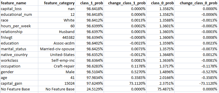
Discussion Of Above
The analysis above follows the same rationale as example 1 above.
The top row shows the overall prediction – namely the probability of this individual earning over $50,000 per annum (Class 1) – of 98.6418%.
So very likely.
In fact, the individual is in Class 1 so the model has made a good prediction.
As it’s the same trained model as example 1, the base Class 1 prediction remains the same at 24.5129%.
Looking down the table shows the impact to the Class 1 probability of removing the feature indicated in the first two columns.
The penultimate row shows that if all one knows about the individual is that their capital_gain is ‘15024’, or $15,024, the probability of being in class 1 moved from the base of 24.5129% to 97.6249%.
Adding the additional information that the age is ’41’ the class 1 probability increases slightly more to 97.9834%.
Similarly, the impact of adding the gender feature value of ‘Male’ moves the class 1 probability higher still to 98.5104% – so very close to the overall prediction of 98.6418%.
The other features are, therefore, irrelevant to the overall prediction.
As a final check, consider the premise that the most important feature is the capital_gain value of ‘$15,024’.
Looking at the training data, there are the 1,399 rows where the capital_gain is over $6,849 and in all number buckets over that value the Class 1 probability ranges from circa 86% to 100%. In the specific bucket covering example 2’s capital_gain of $15,024 there are 493 rows and the Class 1 probability is 100% which explains why the model gave a Class 1 probability of 97.6249%.
The question of feature sensitivity is covered by the sensitivity analysis below.
Feature Sensitivity Analysis Example 1 – Adult Income
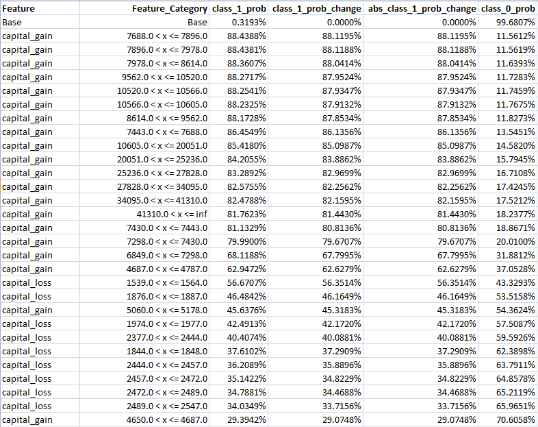
Discussion Of Above
The above shows the top part of the sensitivity analysis for the prediction whose importance analysis was set out above.
The first row shows the base prediction – namely 0.3193%.
The sensitivity analysis was calculated by changing each feature value, one by one, and running the model after each change to determine the impact on the base prediction.
The rows are sorted according to the absolute value change to the class 1 probability.
The analysis shows that certain values of capital_gain and capital_loss could drastically change the prediction.
Feature Sensitivity Analysis Example 2 – Adult Income
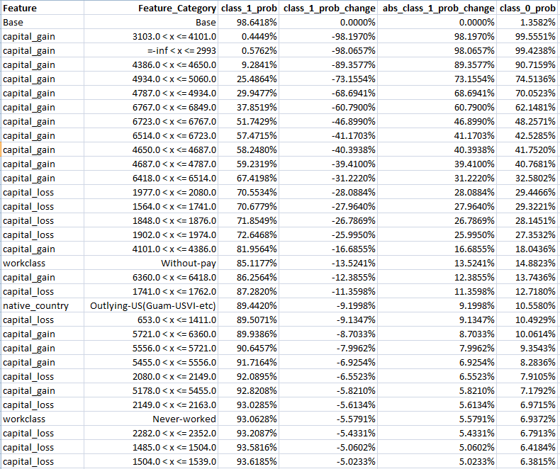
Discussion Of Above
The above shows the top part of the sensitivity analysis for the prediction whose importance analysis was set out above.
The first row shows the base prediction – namely 98.6418%.
The sensitivity analysis was calculated by changing each feature value, one by one, and running the model after each change to determine the impact on the base prediction.
The rows are sorted according to the absolute value change to the class 1 probability.
The analysis shows that certain values of capital_gain and capital_loss could drastically change the prediction.
Model Test Probabilities vs Test Label Probabilities
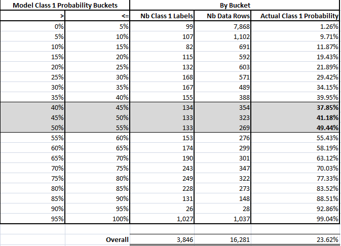
Discussion Of Above
One of the difficulties of assessing the probabilities created by a classification model is that the labels are class labels and not probabilities.
This contrasts with regression models where the output produced by the model can be compared directly to the target value.
AIBMod wanted to try and ascertain the likelihood that when the model produces a Class 1 probability in the high 90s or in the low single digits it represented a ‘real’ probability and not just an ‘artefact’.
AIBMod realised that if the test model probabilities were sorted into 5% buckets the proportion of the Class 1 labels within those buckets should, broadly speaking, fit within the bucket boundaries.
The table above shows the results of this analysis.
Broadly speaking, the analysis shows that at the extremes the model output test probabilities result is label 1 frequencies match very well. Other than the three highlighted buckets the realised label 1 frequencies fit within the 5% probability buckets.
The model may be relatively better at the extremities because of the way the loss function functions – in the case of binary cross entropy it’s always comparing to the class labels of either 0 or 1.
There is a further breakdown of the extremities below, splitting the 0% – 5% and 95% – 100%buckets into 1% buckets.
Model Test Probabilities vs Test Label Probabilities – 1% Buckets
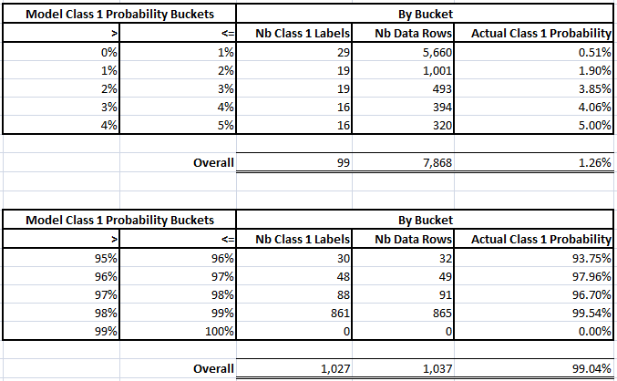
Discussion Of Above
Looking at the 0% – 5% bucket breakdown the probabilities match up fairly well.
The highest frequency bucket of 0% to 1% matches very well with the actual observed Class 1 probability of 0.51%.
Looking at the 95% – 100% bucket breakdown the performance is not as strong as for the 0% – 5% breakdown but that may be driven partially by the low frequency of events within those buckets.
Another observation is that the model did not predict anything in the 99% to 100% bucket – in fact looking at the prediction probabilities the maximum value for Class 1 probability was 98.677%.